Calculation of diversification indicators and other covariates
Summary
Indicators
| Indicator | Data | Format |
|---|---|---|
| perimeter and area of the field | RPG | vectoriel |
| hedgerows length around field | RPG + BD haies | vectoriel |
| mean field size within buffer | RPG | vectoriel |
| crop rotation (N-5:N) | RPG + OSO | raster |
| % land cover within buffer | RPG + OSO | raster |
| edge density | RPG + OSO | raster |
Datasets
Registre Parcellaire Graphique (RPG)(45Gb): annual field crop data for the period 2007-2024 available at France scale on IGN website: https://geoservices.ign.fr/rpg. Definition of field (parcelles) are coherent only in the recent period 2015-2023.
Carte d’occupation des sols du CES OSO – THEIA (OSO)(6.6Gb): annual land cover data for the period 2016-2024. Available for France in raster format and 10m resolution https://doi.org/10.57745/UZ2NJ7. Official access through the CNES website https://geodes-portal.cnes.fr.
BD Haies v2 (6.8Gb): hedgerows dataset for France available on the IGN website: https://geoservices.ign.fr/bdhaie. BD Haie v2 was produced from satellite images of 2020-2022 (which is a better fit to our data than v1 from images of 2011-2014).
RPG complété: add missing crop field data that was not officially reported in the Common Agricultural Policy (PAC in French acronym) so absent from the
RPGdataset. It uses a combination of datasets from cadastre, IGN BD TOPO and OSO. Data is publicly available for the period 2018-2023 and it could be retrieve for the year 2016-2017 directly from Pierre Cantelaube (INRAE - ODR). The year 2024 will not be available in time for our project. The dataset is stored in multiple files per year and per regions or department https://entrepot.recherche.data.gouv.fr/dataverse/rpg_complete_2022. The main issue is that the definition of parcelle inRPGis different from cadastre inRPG complété, so it may bring biases in the vectorial calculations (based on the field definition). Additionally, it is heavy to process (download hundreds of files, merge them per year, ensure consistent classes with RPG) and it might bring only limited information on land cover. For this first exploration, RPG complété was not included but the discussion is open.Land cover class harmonization: list all classes from RPG and OSO and categorize them. This file must be double checked by expert and customized for the project objectives.
Field observations
| 2014 | 2015 | 2016 | 2017 | 2018 | 2019 | 2020 | 2021 | 2022 | 2023 | 2024 | TOTAL | |
|---|---|---|---|---|---|---|---|---|---|---|---|---|
| BACCHUS | 0 | 0 | 0 | 0 | 40 | 38 | 40 | 40 | 38 | 38 | 38 | 272 |
| BIOMHE | 0 | 0 | 0 | 0 | 0 | 0 | 40 | 0 | 0 | 0 | 0 | 40 |
| BISCO | 0 | 0 | 0 | 27 | 0 | 0 | 0 | 0 | 0 | 0 | 0 | 27 |
| DIVAG | 0 | 0 | 0 | 0 | 0 | 40 | 0 | 0 | 0 | 0 | 0 | 40 |
| DURUM_MIX_GM | 0 | 0 | 0 | 1 | 1 | 0 | 0 | 0 | 0 | 0 | 0 | 2 |
| FRAMEwork_BVD | 0 | 0 | 0 | 0 | 0 | 0 | 0 | 36 | 0 | 0 | 0 | 36 |
| LepiBats | 0 | 0 | 0 | 0 | 0 | 0 | 0 | 50 | 0 | 0 | 0 | 50 |
| MUESLI | 0 | 0 | 60 | 0 | 0 | 0 | 0 | 0 | 0 | 0 | 0 | 60 |
| OSCAR | 0 | 0 | 0 | 0 | 15 | 33 | 38 | 67 | 88 | 100 | 107 | 448 |
| SEBIOPAG_BVD | 0 | 0 | 0 | 0 | 0 | 0 | 20 | 20 | 20 | 0 | 0 | 60 |
| SEBIOPAG_Plaine de Dijon | 20 | 20 | 20 | 20 | 20 | 20 | 20 | 20 | 20 | 20 | 20 | 220 |
| SEBIOPAG_VcG | 19 | 19 | 17 | 17 | 17 | 17 | 17 | 17 | 17 | 17 | 0 | 174 |
| SEBIOPAG_ZAAr | 20 | 20 | 20 | 0 | 20 | 0 | 0 | 20 | 0 | 20 | 0 | 120 |
| SERIPAGE | 0 | 0 | 9 | 0 | 0 | 0 | 0 | 0 | 0 | 0 | 0 | 9 |
| TOTAL | 59 | 59 | 126 | 65 | 113 | 148 | 175 | 270 | 183 | 195 | 165 | 1558 |
Indicators from vector datasets
Identification of the crop field in RPG
Because of data availability, we will only focus on the observations made in the period 2016-2023 (N=1275). RPG 2024 was only released at the end of November 2025 and is not included yet.
We identified the crop field from RPG dataset corresponding to the observations based on the coordinates and the year of the samplings.
| Nobs | in_RPG | Perc | |
|---|---|---|---|
| BACCHUS | 234 | 189 | 80.77 |
| BIOMHE | 40 | 39 | 97.50 |
| BISCO | 27 | 26 | 96.30 |
| DIVAG | 40 | 40 | 100.00 |
| DURUM_MIX_GM | 2 | 0 | 0.00 |
| FRAMEwork_BVD | 36 | 30 | 83.33 |
| LepiBats | 50 | 30 | 60.00 |
| MUESLI | 60 | 31 | 51.67 |
| OSCAR | 341 | 312 | 91.50 |
| SEBIOPAG_BVD | 60 | 51 | 85.00 |
| SEBIOPAG_Plaine de Dijon | 160 | 160 | 100.00 |
| SEBIOPAG_VcG | 136 | 48 | 35.29 |
| SEBIOPAG_ZAAr | 80 | 80 | 100.00 |
| SERIPAGE | 9 | 9 | 100.00 |
In total, 82 % of the fields observations are covered by RPG data. There are large disparities among projects with SEBIOPAG_VcG, MUESLI and LepiBats having a lower coverage than 60%. The project DURUM_MIX_GM has only one coordinates leading to the entrance of the Institut Agro-Montpellier.
To be discussed:
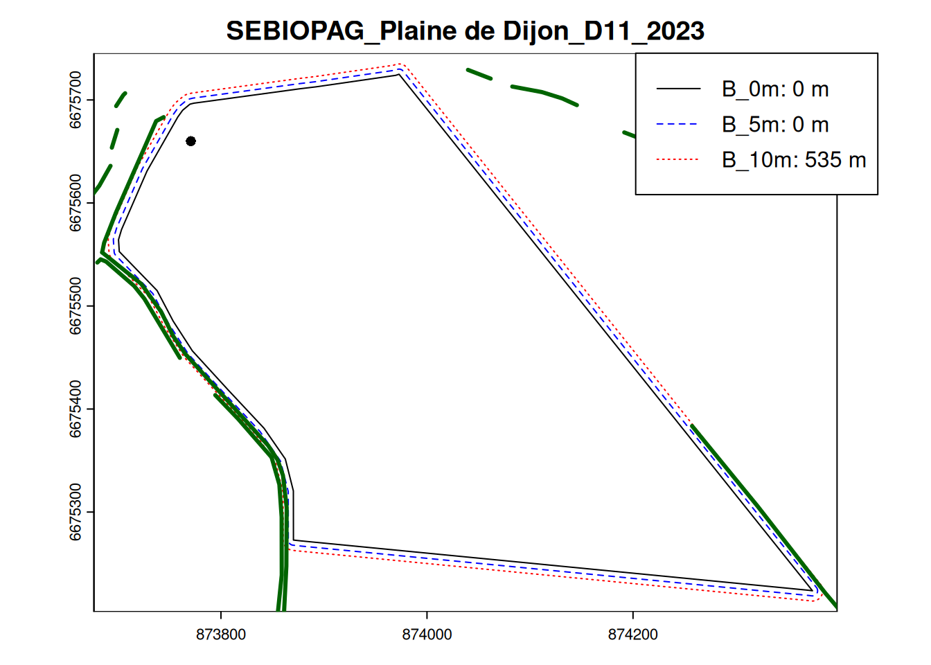
- Some coordinates were taken at the edge or on the boundary of the field (Figure 3), so it is not possible to clearly identify in which field they belong. In such case, using RPG complété will probably not help. Should we consider the closest field within a distance threshold (e.g. 10m)?
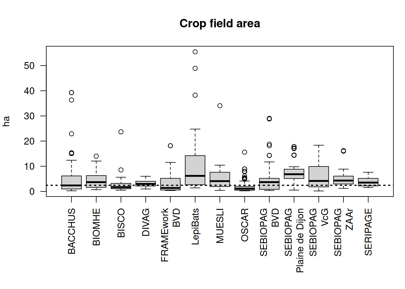
Field size
We calculated the area and the perimeter of the crop fields corresponding to the samplings.
| Min. | 1st Qu. | Median | Mean | 3rd Qu. | Max. | |
|---|---|---|---|---|---|---|
| BACCHUS | 0.26 | 0.98 | 2.38 | 4.52 | 6.16 | 39.27 |
| BIOMHE | 0.68 | 1.59 | 3.69 | 4.48 | 6.29 | 13.99 |
| BISCO | 0.50 | 1.10 | 1.71 | 3.22 | 3.15 | 23.69 |
| DIVAG | 0.97 | 2.21 | 2.98 | 3.17 | 4.02 | 6.01 |
| FRAMEwork_BVD | 0.36 | 0.56 | 1.36 | 3.83 | 5.01 | 18.15 |
| LepiBats | 1.40 | 2.77 | 6.18 | 11.89 | 13.96 | 55.47 |
| MUESLI | 0.41 | 1.91 | 4.10 | 5.64 | 7.61 | 34.05 |
| OSCAR | 0.23 | 0.48 | 1.10 | 1.71 | 1.96 | 15.60 |
| SEBIOPAG_BVD | 0.36 | 0.83 | 3.68 | 5.70 | 5.20 | 29.02 |
| SEBIOPAG_Plaine de Dijon | 0.53 | 5.11 | 6.83 | 7.41 | 8.78 | 17.82 |
| SEBIOPAG_VcG | 0.19 | 1.82 | 4.16 | 6.40 | 9.90 | 18.35 |
| SEBIOPAG_ZAAr | 1.21 | 2.96 | 4.31 | 4.83 | 6.09 | 16.22 |
| SERIPAGE | 1.55 | 2.19 | 3.51 | 4.04 | 5.19 | 7.60 |
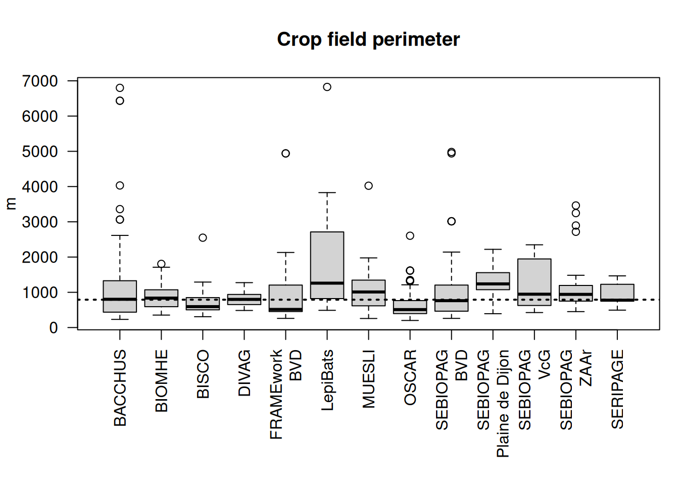
| Min. | 1st Qu. | Median | Mean | 3rd Qu. | Max. | |
|---|---|---|---|---|---|---|
| BACCHUS | 231.16 | 436.43 | 801.76 | 1082.18 | 1328.44 | 6800.54 |
| BIOMHE | 353.82 | 591.74 | 835.19 | 907.14 | 1071.40 | 1805.91 |
| BISCO | 307.43 | 503.79 | 593.37 | 742.83 | 846.60 | 2549.66 |
| DIVAG | 485.10 | 654.49 | 799.27 | 815.71 | 937.28 | 1274.27 |
| FRAMEwork_BVD | 259.84 | 456.32 | 514.18 | 1009.96 | 1130.44 | 4941.28 |
| LepiBats | 488.27 | 823.78 | 1260.07 | 1788.52 | 2669.29 | 6826.56 |
| MUESLI | 257.40 | 616.49 | 1008.85 | 1095.07 | 1345.82 | 4023.55 |
| OSCAR | 201.16 | 397.01 | 509.85 | 599.83 | 764.15 | 2604.84 |
| SEBIOPAG_BVD | 259.84 | 464.35 | 763.05 | 1135.47 | 1205.33 | 4981.42 |
| SEBIOPAG_Plaine de Dijon | 393.18 | 1074.23 | 1239.00 | 1290.33 | 1557.35 | 2219.05 |
| SEBIOPAG_VcG | 425.74 | 626.06 | 945.93 | 1230.81 | 1946.87 | 2347.86 |
| SEBIOPAG_ZAAr | 451.68 | 750.06 | 941.04 | 1030.21 | 1188.23 | 3463.63 |
| SERIPAGE | 494.16 | 750.32 | 776.33 | 927.95 | 1227.07 | 1465.95 |
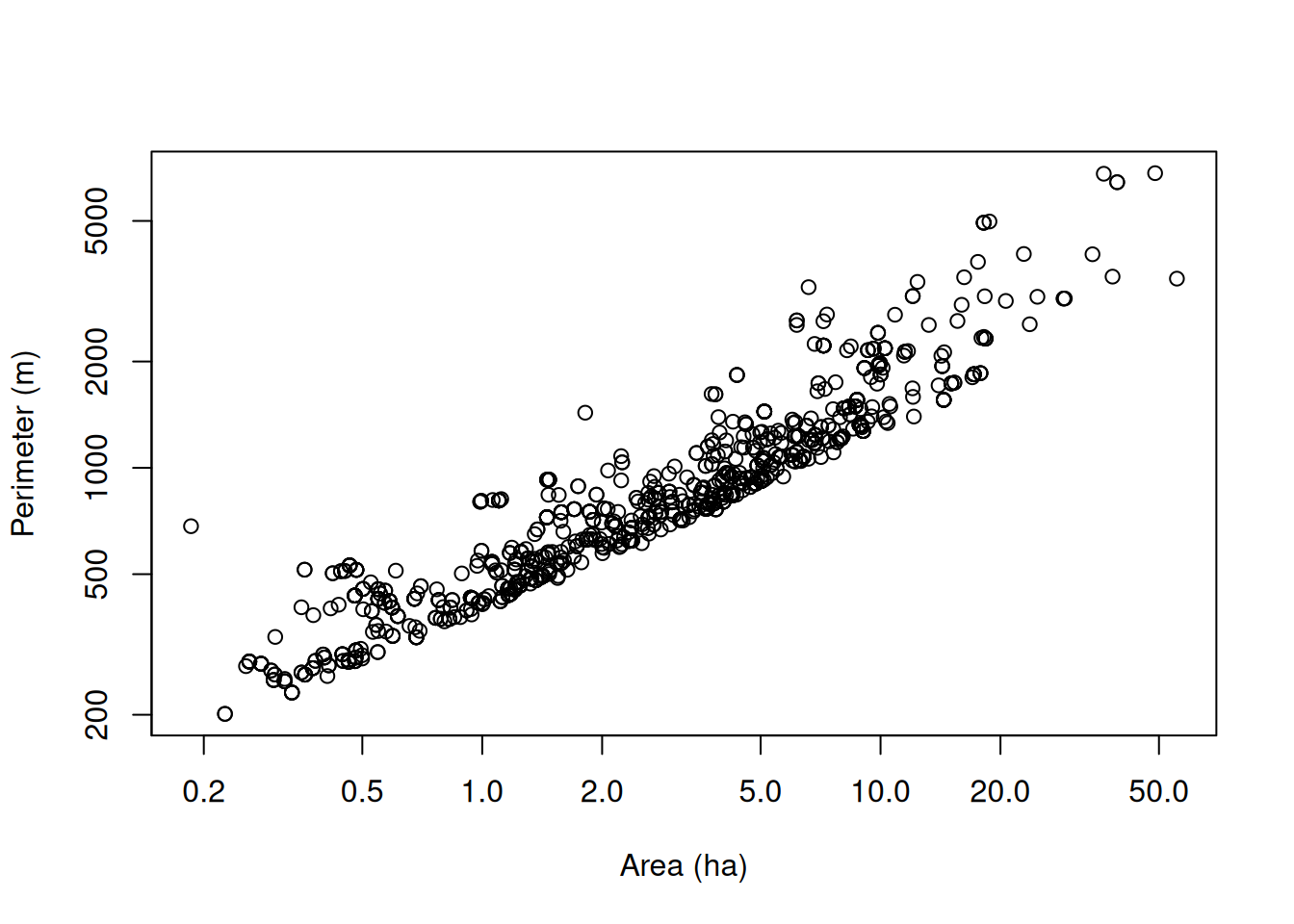
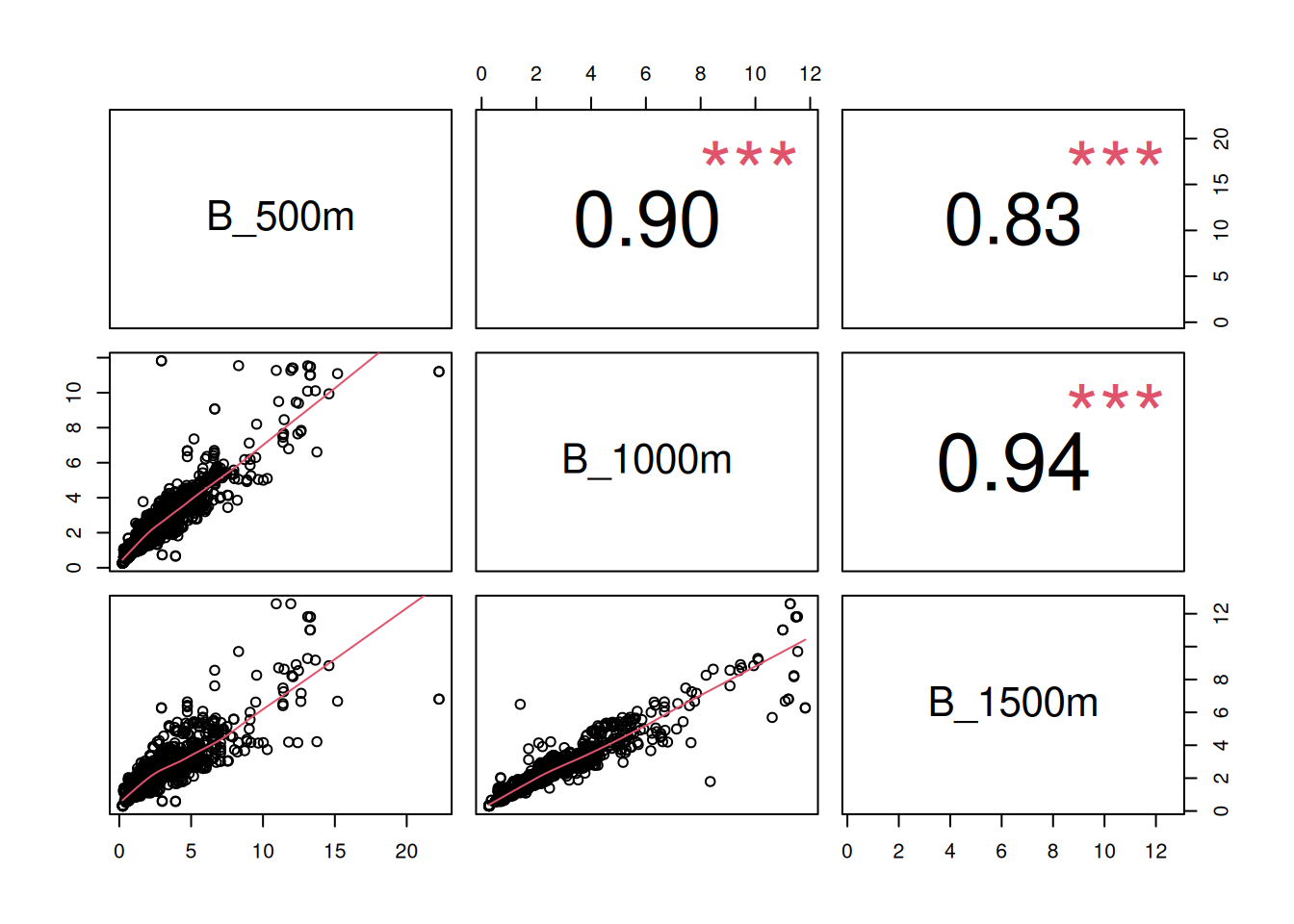
There is a strong relation between area and perimeter (Figure 6). In median, field size is 2.8 ha and field perimeter is 790m.
Outliers
To be discussed:
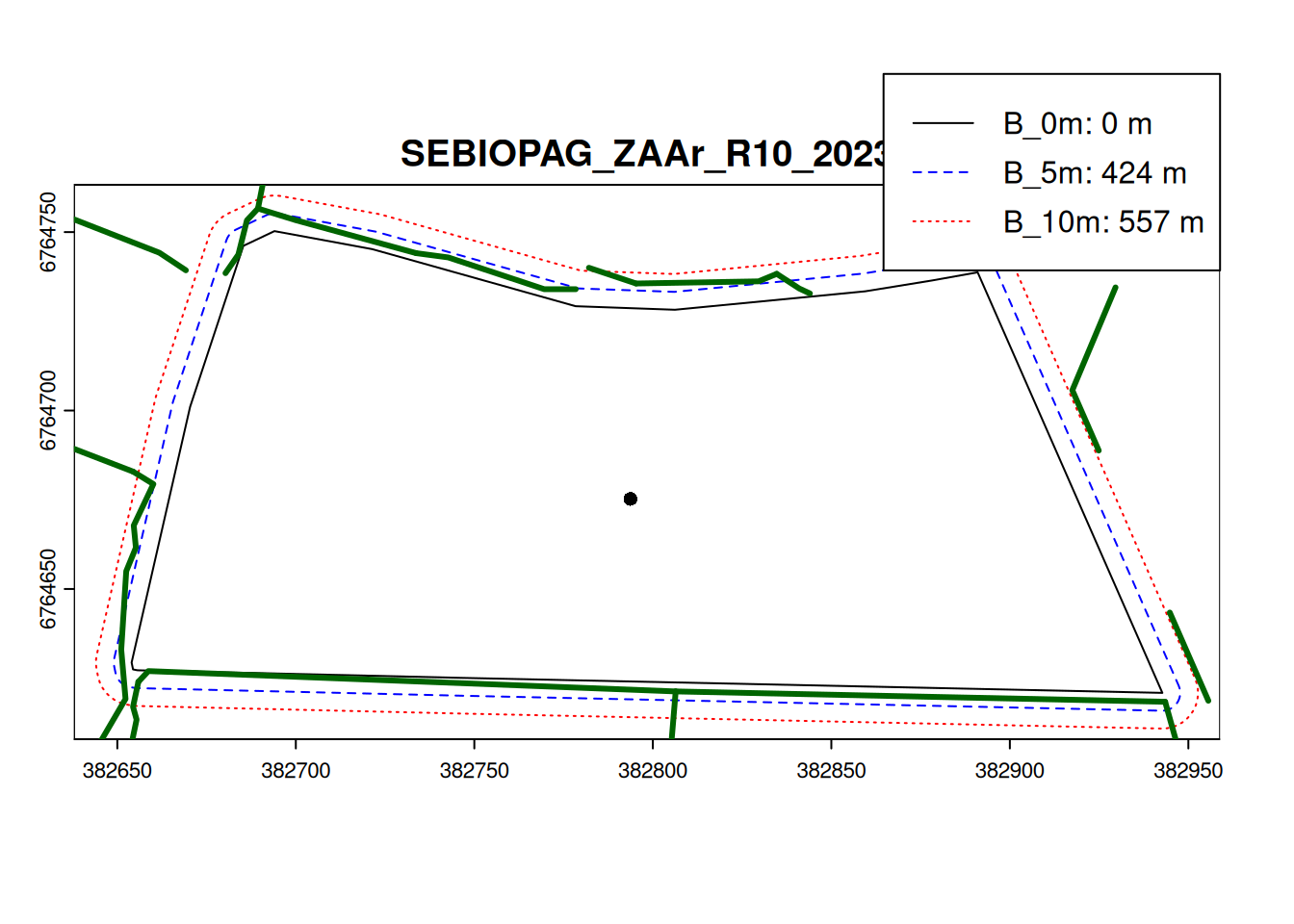
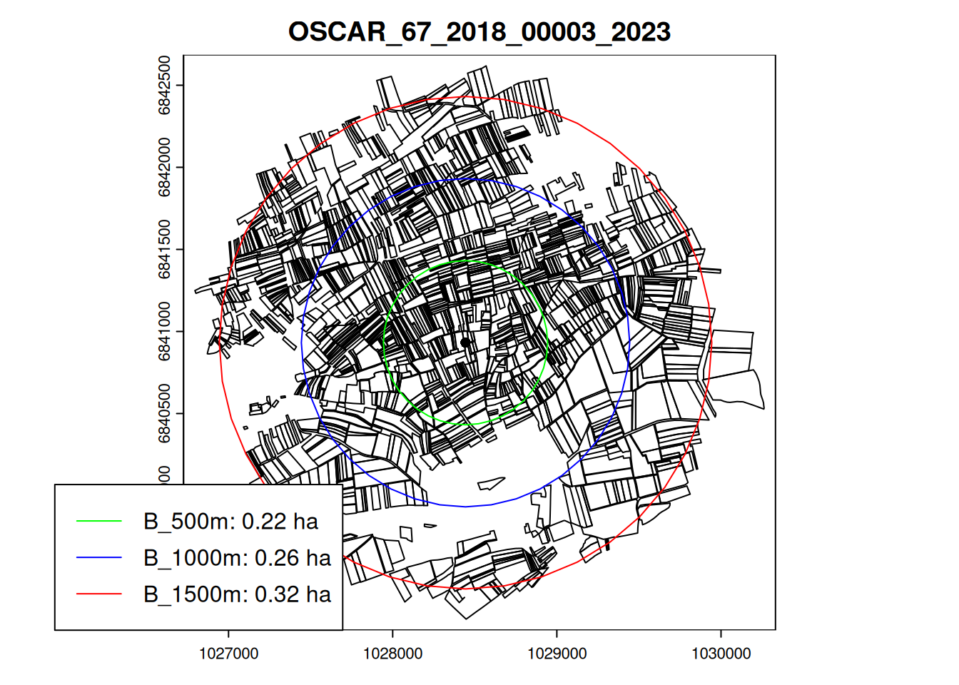
- Some fields are defined as
Bordure de champwhich are not proper fields but borders (as in Figure 8). Should we remove non crop fields from RPG before running the calculations (e.g.Bordure,Bande tampon,Surface non agricole,Truffière,Bois paturés)?
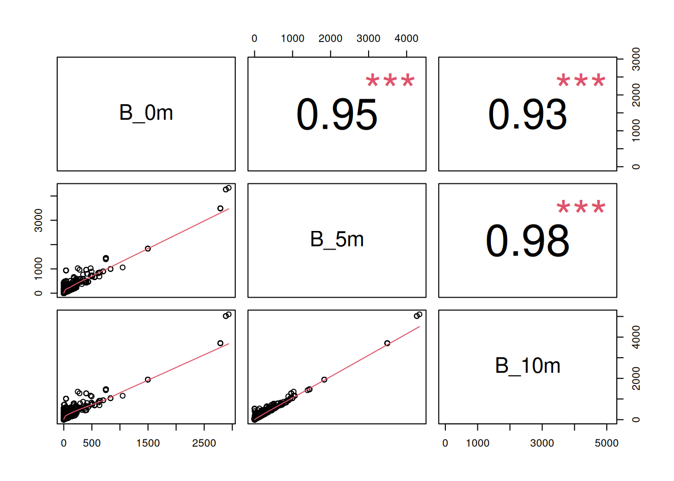
Hedgerows length
Using the field as defined in RPG, we calculated the length of hedgerows from BD Haies that intersect the field (+ a small buffer).
| B_0m | B_5m | B_10m | |
|---|---|---|---|
| Min. | 0.00 | 0.00 | 0.00 |
| 1st Qu. | 0.00 | 0.00 | 0.00 |
| Median | 0.00 | 30.97 | 68.36 |
| Mean | 82.00 | 167.59 | 213.70 |
| 3rd Qu. | 51.00 | 201.30 | 288.28 |
| Max. | 2935.23 | 4336.95 | 5105.47 |
| NA’s | 230.00 | 230.00 | 230.00 |
| PercWithHedgerows | 42.11 | 60.00 | 70.14 |
The 230 NA’s correspond to the observations from which no corresponding fields were found. Without buffer, 42% of fields have hedgerows within the field. This percentage increases up to 70% if we consider a 10m buffer around the field.
Outliers
To be discussed:
- Which buffer size should we use to calculate the hedgerows lengths? Without buffer, it might be too restrictive, but is 10m too large, or not enough?
- Should we consider the location of the sampling when calculating the hedgerows length?
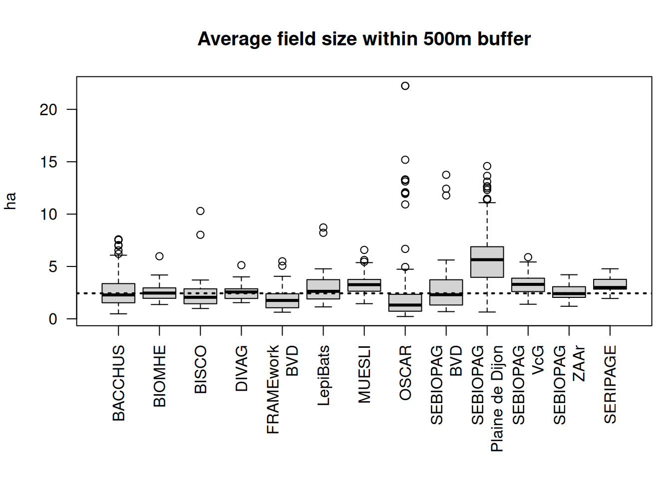
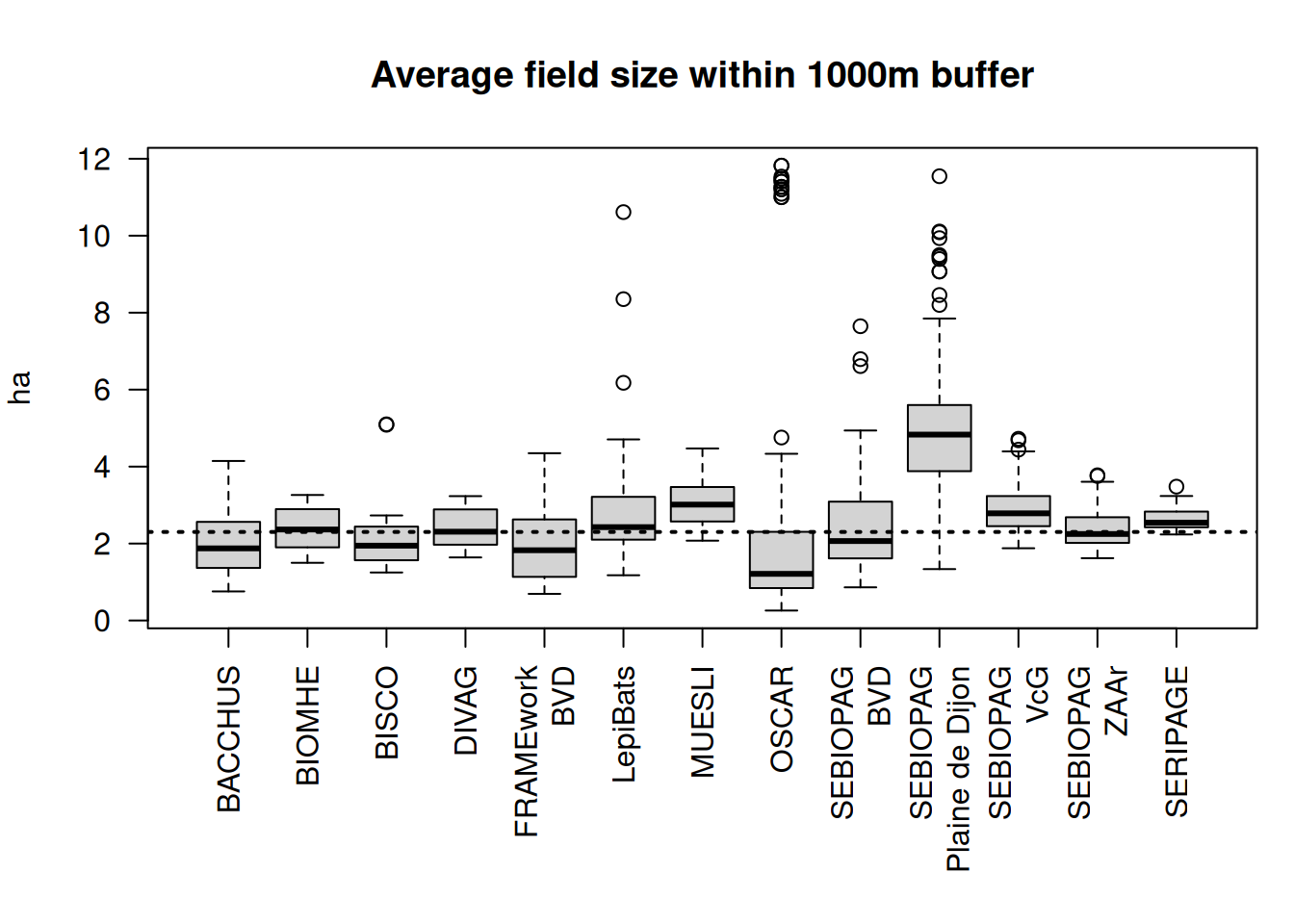
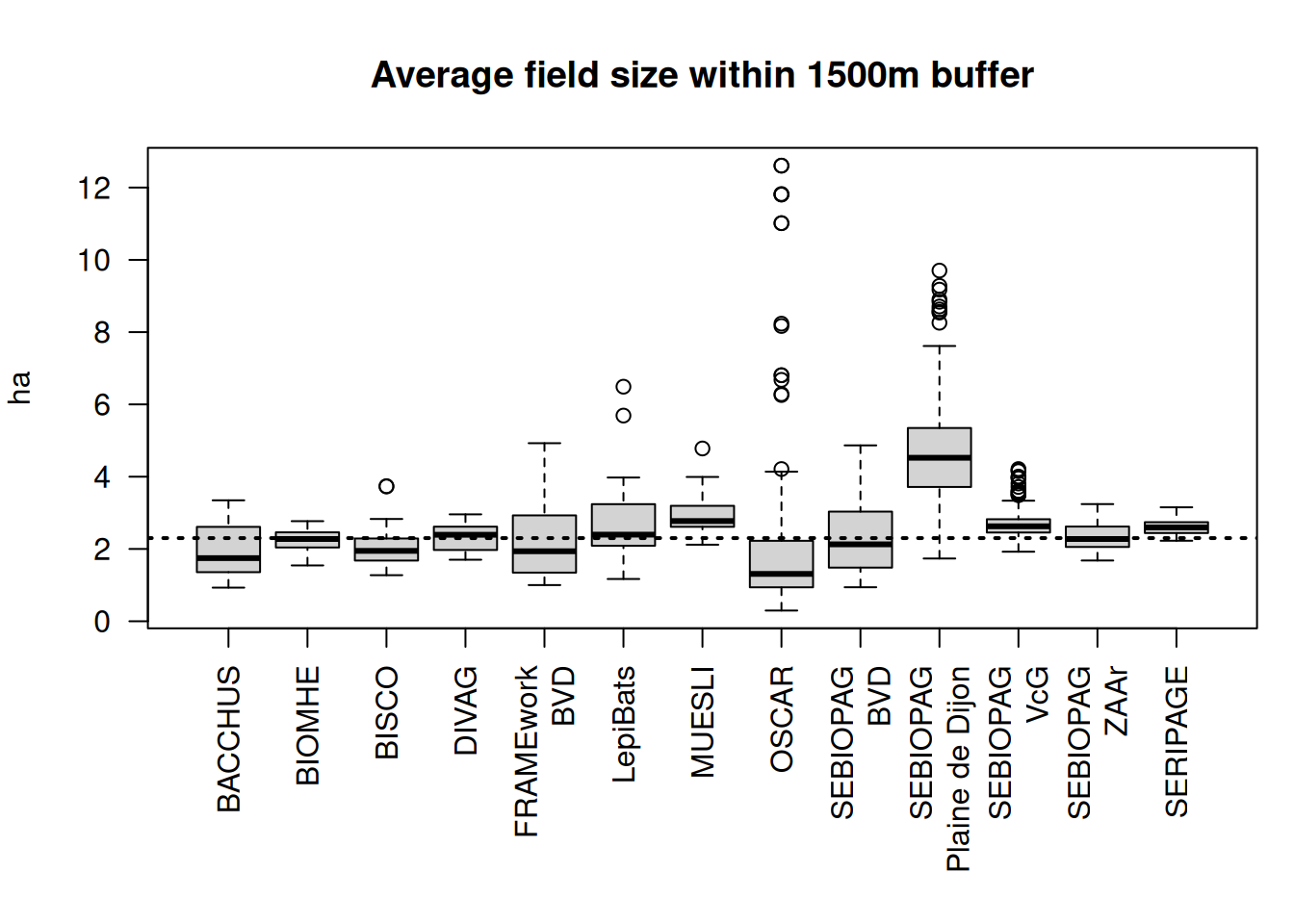
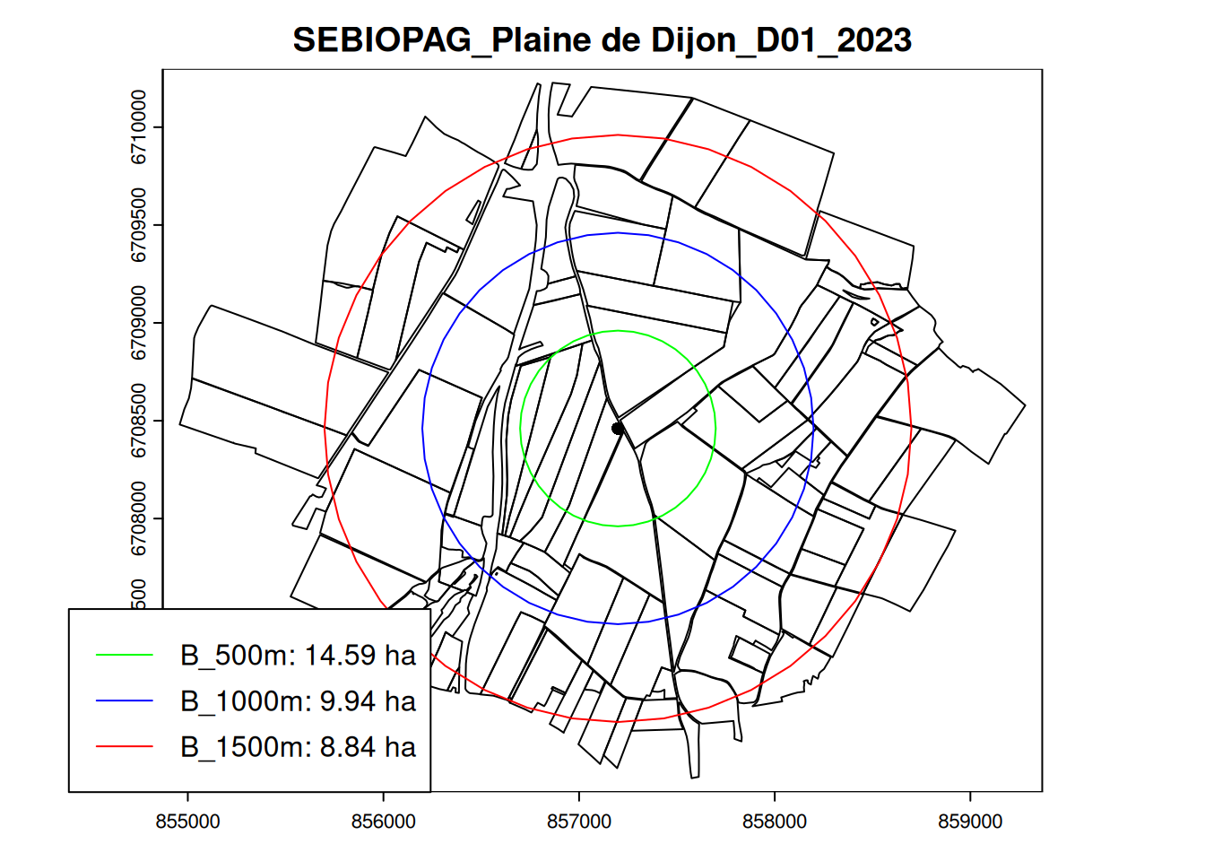
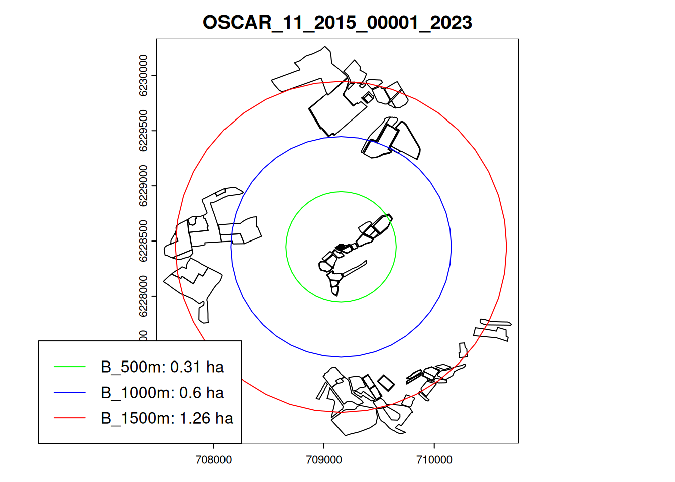
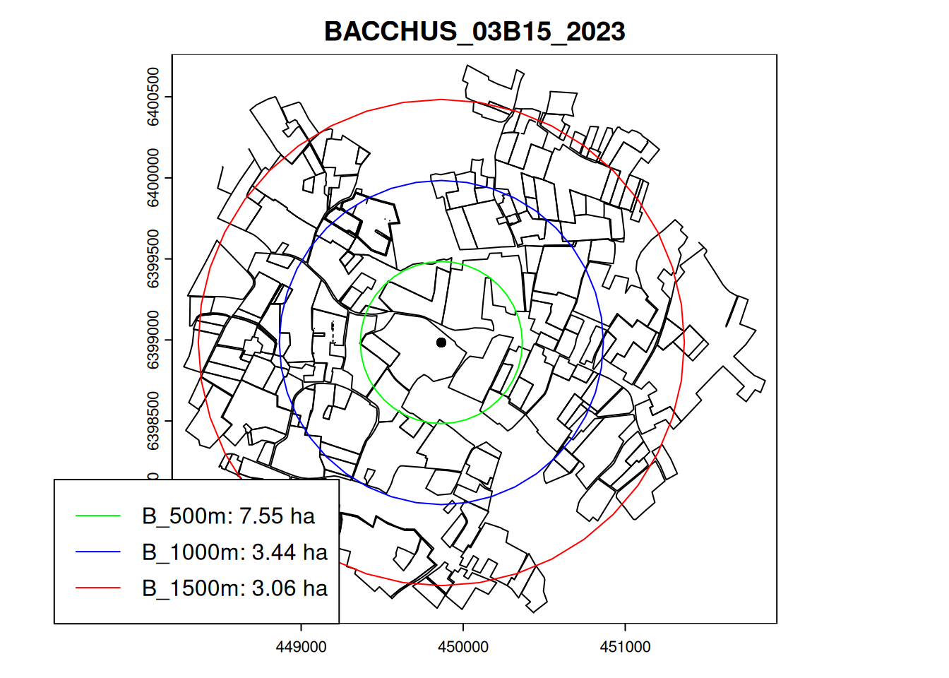
Field size within buffer
Using the coordinates of the sampling sites, we calculated the average area of all crop fields within a buffer (500m, 1000m, and 1500m).
| B_500m | B_1000m | B_1500m | |
|---|---|---|---|
| Min. | 0.22 | 0.26 | 0.30 |
| 1st Qu. | 1.50 | 1.57 | 1.55 |
| Median | 2.44 | 2.33 | 2.30 |
| Mean | 3.00 | 2.63 | 2.51 |
| 3rd Qu. | 3.69 | 3.15 | 2.93 |
| Max. | 22.25 | 11.82 | 12.61 |
| NA’s | 13.00 | 7.00 | 5.00 |
We see that some observations don’t have crop field within 500m (N=13). These observations (listed in Table 7) would need to be checked and ensure that they are close to an agricultural field.
| Study_ID | Site | Year | |
|---|---|---|---|
| 154 | DURUM_MIX_GM | DIASCOPE | 2017 |
| 232 | DURUM_MIX_GM | DIASCOPE | 2018 |
| 704 | LepiBats | C01 | 2021 |
| 705 | LepiBats | C02 | 2021 |
| 706 | LepiBats | C03 | 2021 |
| 707 | LepiBats | C04 | 2021 |
| 708 | LepiBats | C05 | 2021 |
| 709 | LepiBats | C06 | 2021 |
| 710 | LepiBats | C07 | 2021 |
| 712 | LepiBats | C09 | 2021 |
| 713 | LepiBats | C10 | 2021 |
| 242 | OSCAR | 33_2011_00002 | 2018 |
| 1133 | OSCAR | 11_2023_00004 | 2023 |
Outliers
Summary and questions about vector indicators
- Most observations have a corresponding crop field in RPG dataset (Table 2).
- But some coordinates were taken at the outside edge of the field (Figure 3), so we might need to identify the closest field instead (and add a distance threshold, e.g. 10m).
- Adding the
RPG complétérequires more data processing and it won’t cover all observations (but it will help characterizing some wineyards that are not registered in the PAC). TheRPG complétéclasses might be less consistent within our timeframe (e.g. issue with data from 2016-2017) so it would require further checks. - We might need to exclude some fields from RPG (e.g.
Bordure,Bande tampon,Surface non agricole,Truffière,Bois paturés) to includes only crop fields that are relevant for us. This information should be added in the file RPG-OSO_classes.csv. - The sampling location within the field might influence the results (different impact of hedgerows, or of agricultural practices). We might want to add an indicator reflecting the distance to the center of the field and/or the distance to the closest field boundary?
Indicators from raster datasets (RPG+OSO)
Annual rasters with a 10m spatial resolution were created based on (1) RPG information and, where missing, (2) OSO dataset. We used these RPG+OSO rasters to extract information on crop rotation, land cover within buffer and edge density.
Crop rotation (N-5:N)
| inRPG | inOSO | NAs | |
|---|---|---|---|
| lulc_N | 1042 | 233 | 283 |
| lulc_N-1 | 1100 | 214 | 244 |
| lulc_N-2 | 1028 | 221 | 309 |
| lulc_N-3 | 923 | 213 | 422 |
| lulc_N-4 | 779 | 209 | 570 |
| lulc_N-5 | 632 | 181 | 745 |
The number of NAs in Table 8 is a results of the number of observations per year (Table 1). For instance at year N, there are NAs for observations carried out in 2014, 2015, and 2024. For year N-1, the NAs correspond to observations carried out in 2014, 2015, and 2016.
| landcover class | N |
|---|---|
| RPG_Vigne (sauf vigne rouge) | 484 |
| RPG_Blé tendre d’hiver | 165 |
| RPG_Autre verger (y compris verger DOM) | 79 |
| OSO_Vignes | 64 |
| OSO_Forêts de feuillus | 41 |
| OSO_Prairies | 41 |
| RPG_Maïs (hors maïs doux) | 34 |
| RPG_Orge d’hiver | 29 |
| RPG_Maïs ensilage | 26 |
| RPG_Mélange de céréales ou pseudo-céréales d’hiver entre elles | 25 |
| RPG_Vigne : raisins de cuve non en production | 24 |
| RPG_Colza d’hiver | 21 |
Vigne is the most common land cover (Table 9), but the information might come from RPG (two classes: Vigne (sauf vigne rouge) and Vigne : raisins de cuve non en production) or OSO. The land cover depends greatly on the project (Figure 20) with OSCAR and BACCHUS studying wineyards, FRAMEwork and SBIOPAG studying orchard, and the other projects focusing on annual crops.
Let’s have a look at the crop rotations over the 6-year period (N:N-5).
There are 648 observations with complete time series from year N to N-5 (Figure 21). From these observations with complete crop rotation information, 342 have the same crop group for the whole time period, while 74 fields have four different crop groups in the past 6 years (Figure 22).
Land cover within buffer
| buffer_500 | buffer_1000 | buffer_1500 | |
|---|---|---|---|
| n_classes | 186 | 220 | 237 |
| av_perc_rpg | 50 | 47 | 45 |
Without any grouping, there are 237 different categories covered by the 1500m buffers (Table 10). Theses categories need to be simplified before the land cover can be analyzed. The larger the buffer size, the higher is the number of different classes within the buffer.
In average, roughly half of the buffer areas are filled with land cover classes from RPG (and the other half are OSO classes). The proportion of RPG classes slightly decreases with the size of the buffer (larger buffer includes less agricultural areas).
The average land cover within buffers among all observations is not really influenced by the size of the buffer (Figure 24). The coverage are highly dynamics (no studies in wineyards in 2016-2017) so the average land cover do change drastically (Figure 25). Yet some categories (cultures d'été and culture d'hiver) are only present in 2016-2017. A better way to look at land cover is to group them by study.
The land cover averages are highly different per study (Figure 28). The size of the buffer have little influence in the overall pattern. Yet increasing the size of the buffers tends to make the land cover more heterogeneous (higher eveness), the dominant class has a higher coverage with a buffer of 500m than 1500m.
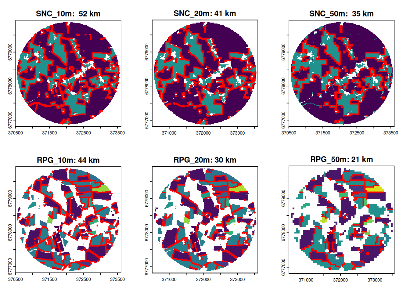
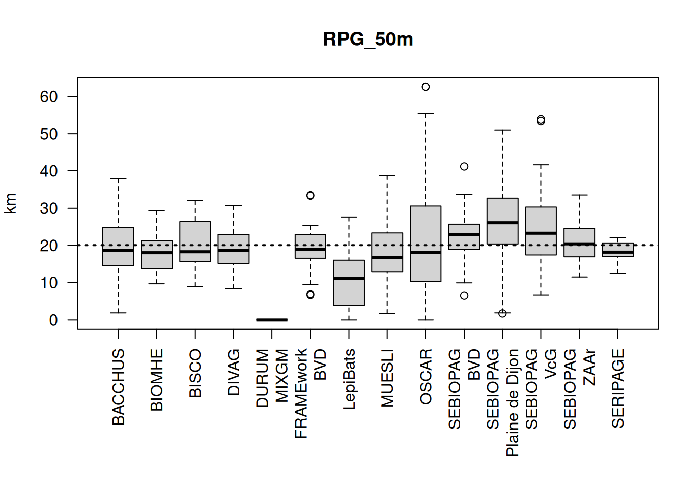
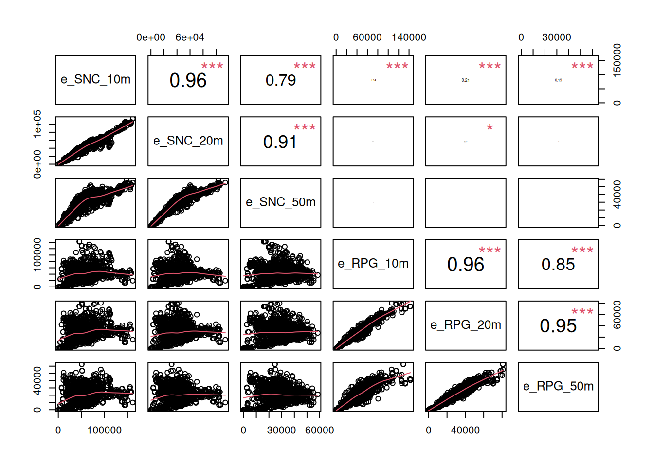
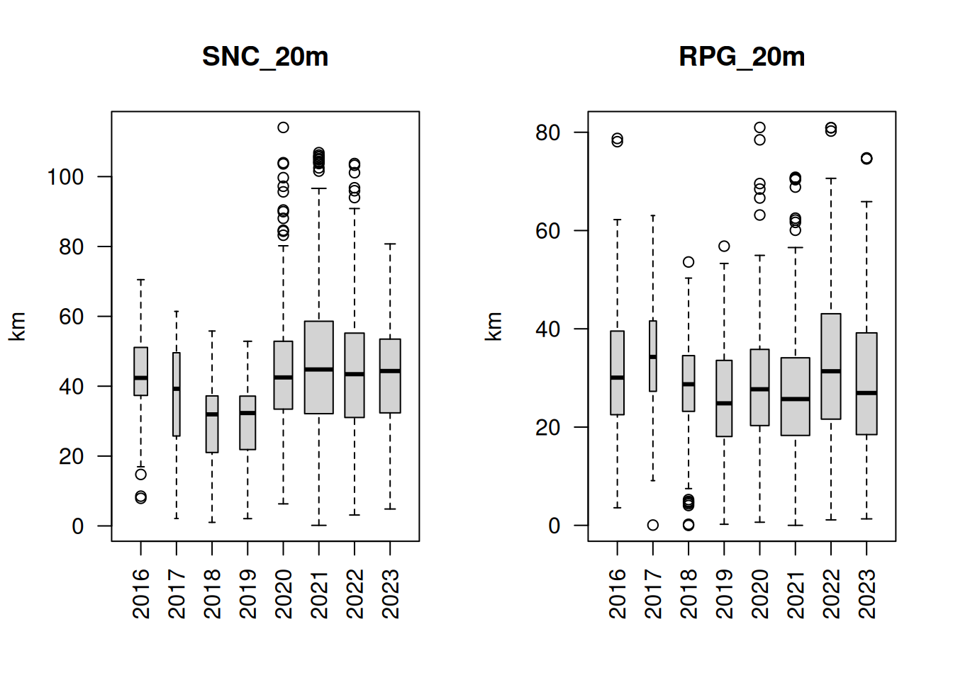
Edge density
This section is still highly exploratory. We considered two different kind of edges:
- SNC: the edges between semi-natural land cover and agricutural crops
- RPG: the edges between different agricultural crops
We calculated the length of the edges within 1500m buffers and using the raster information at 10m, 20m, or 50m resolution.
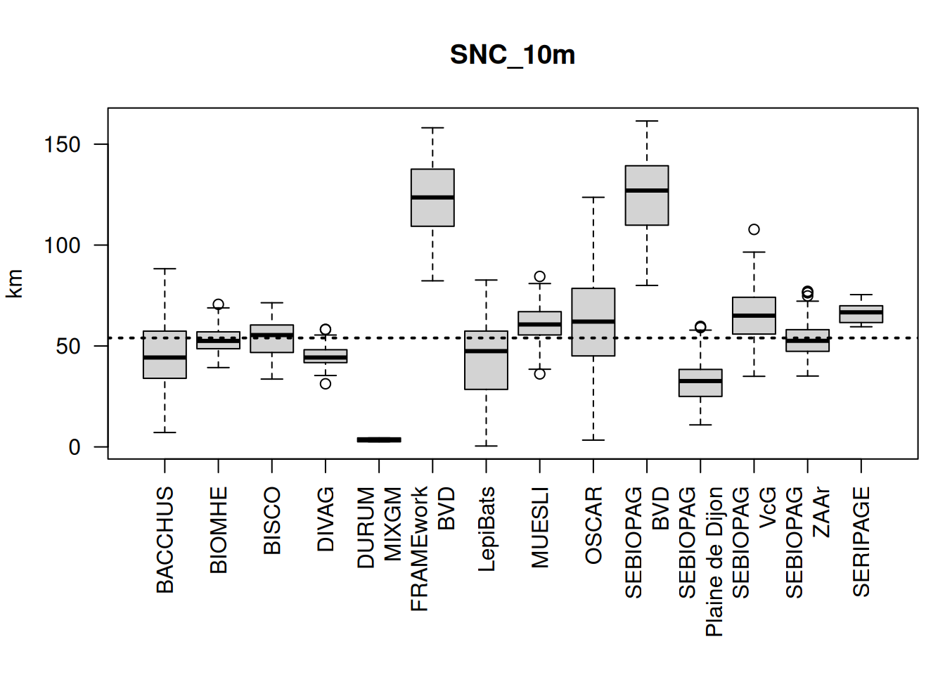
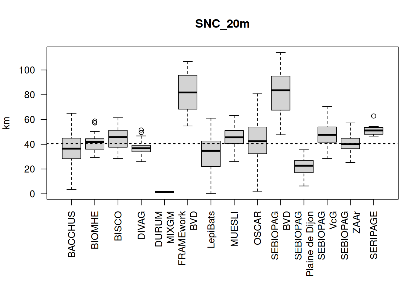
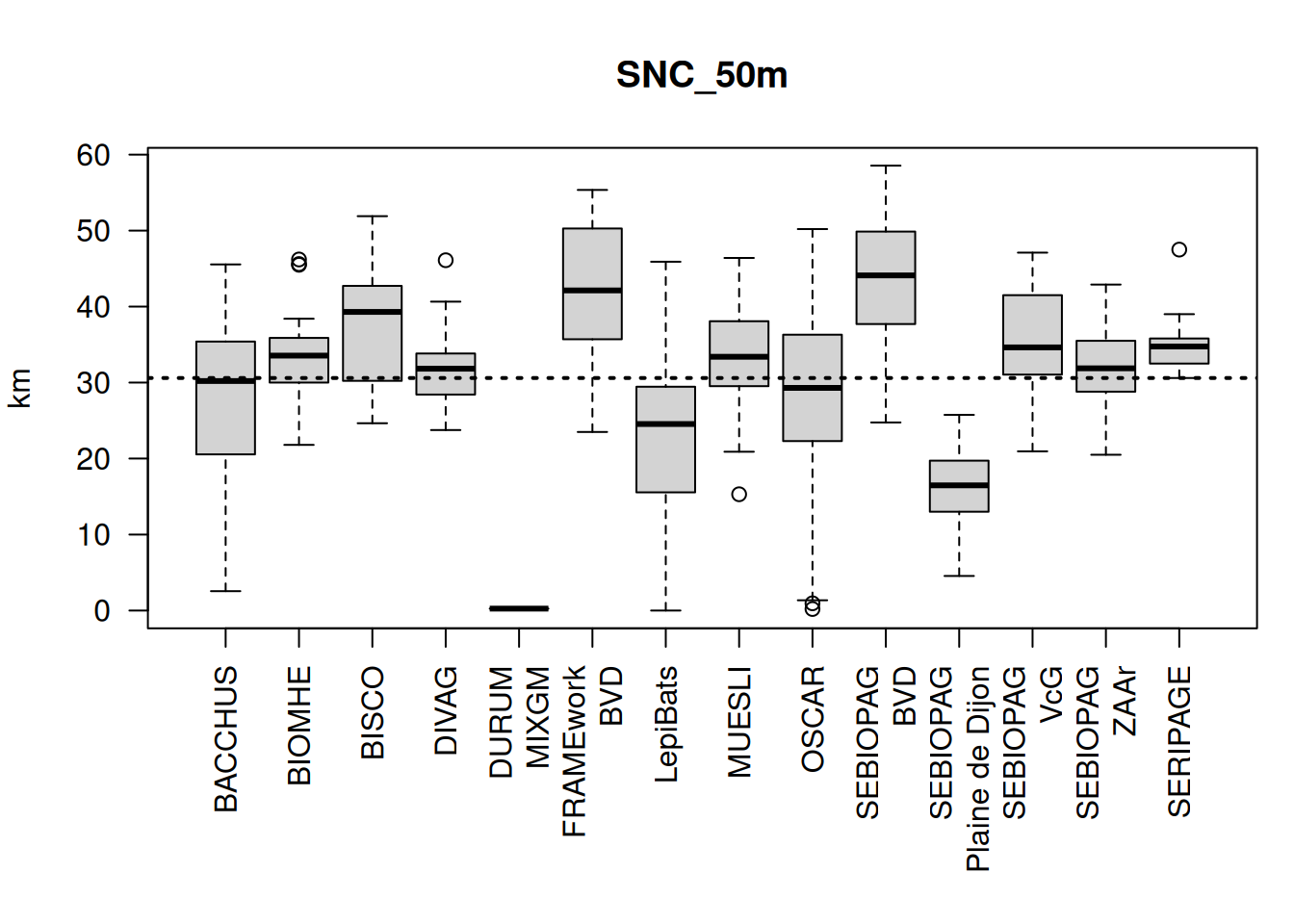
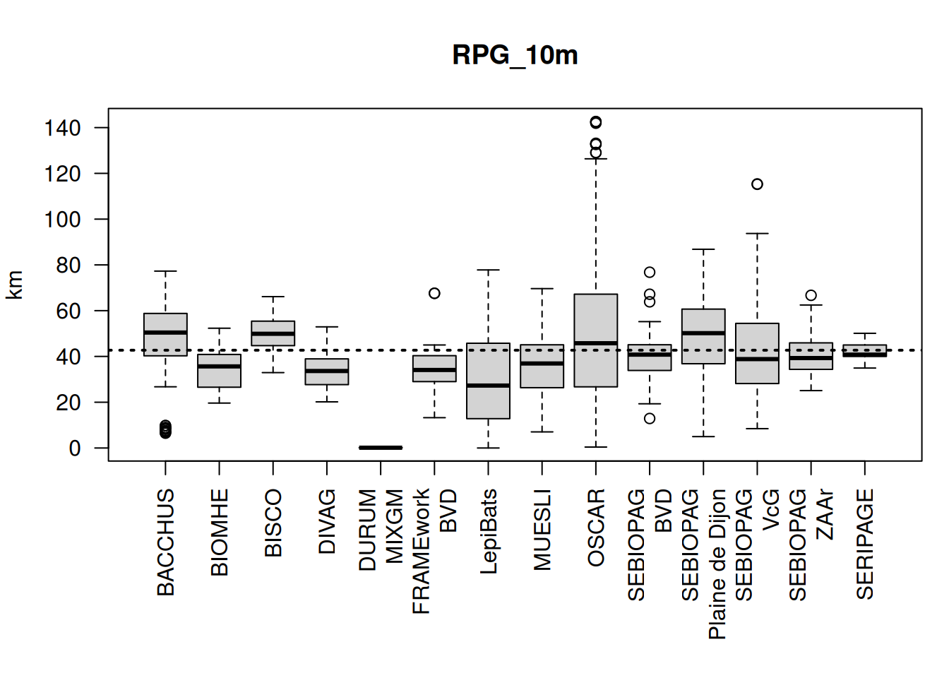
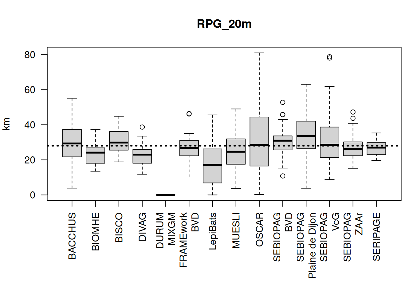
Summary and questions about raster indicators:
Annual rasters combining RPG and OSO for the whole France simplify the extraction of indicators on crop rotations, proportion of land cover within buffers and edge length density.
There are up to
237land cover classes in the RPG+OSO dataset. Here we simplified it using the Référentiel des cultures (36 categories) as an illustration. Further work on land cover class homogeneization is needed to make use of the extracted information. This will be done independantly from the GIS data extraction.The edge density needs further thinking to decide which kind of edges should be quantified, and at what scale. The spatial resolution depends on the minimum size of the patches that we want to consider.
The OSO data for year 2016-2017 use different classes, e.g. crops are grouped into only two classes:
cultures d'étéandculture d'hiver. This might artificially inflate crop rotations (changes in land cover due to changes in GIS methodology instead of changes in crop practices) and it could potentially impact all indicators. Yet it is important to use older land cover if we want to characterize crop rotations on multiple years.We could add
RPG complétéin the land cover rasters, but that might create discrepancies among classes and it would require additional care in the class homogeneization step.The resolution of 10m might be to rough for the caracterization of the crop fields. We might want to consider 5m or 2m spatial resolution (but we are also constrained by OSO).